
This article explores how anyone can train advanced AI models in just a few minutes by employing a technique called transfer learning. This approach allows taking a more generic, complex, pre-trained model and applying it to a more specific use case by only swapping out the model’s topmost layers to better suit a concrete task. Read on to learn more!
This is part two of a mini-series, and I suggest you take a look at part one as well if you haven’t done so already! The first part discusses the pros and cons of cloud-based ML training and how to find suitable data for the process.
Transforming Image Data for Machine Learning
Recall the previous part of this series. We concluded it by uploading and labeling thousands of sample images of cats and dogs, and we let the platform perform a random 80-20 split into the training and test sets.
In this instance, we’re dealing with images of cats and dogs. But that is a human way of looking at the data. A computer doesn’t look at the data like that – it can only handle numeric information. So, the first task of solving any ML problem (or most computational problems in general, for that matter) is to transform the problem into something the machine can understand.
Similarly, we should be aware of how much data we try to stuff into the model. Generally speaking, the greater the amount, the longer training takes and the more complex the resulting model. Finally, neural networks, in particular (the type of model we want to train here), can only deal with inputs of the same size, so we must further ensure that all samples and images to be classified have the same shape (including color channels).
We can break down the images into individual pixels with three intensity values (red, green, and blue). When dealing with 32-bit images, that still leaves us with 16,777,216 possible RGB values per pixel, of which there could be millions in an image. These vectors are too large to deal with efficiently. So before that, we have to resize the images to reduce the amount of data and ensure they all adhere to a uniform shape. Further, we may want to remove the color channels and convert the images to grayscale images before feeding them into the model for training or classification. These steps are referred to as preprocessing, and there can be many more, depending on the specific task.
The Importance of Preprocessing in Transfer Learning
These preprocessing steps become even more critical in transfer learning since you take an already trained model and shave off its topmost layers to replace them with new ones. In doing so, you can leverage the accuracy and robustness of pre-trained models that have seen much more data than you could ever acquire without having to start from scratch. The result is a compromise between accuracy, training time, and customizability. Usually, you should employ transfer learning for standard problems whenever possible, especially if you’re new to building (computer vision) models, because building one from scratch and ensuring it works well in different real-life conditions is very laborious and challenging. The process requires many samples taken from different angles, lighting conditions, etc., to ensure that the resulting model generalizes well. All of that knowledge is already encoded in pre-trained models such as MobileNet.
As mentioned above, the data must adhere to a specific format to be compatible with a neural network. Since we’re not building one from scratch, we must ensure that our data samples follow the expected format of the base model used for transfer learning. In this instance, we’ll use MobileNetV2 96x96, meaning our images should be 96x96 pixels in size and supplied as grayscale or RGB images. Other variations may have different requirements (e.g., just MobileNetV2 with 160x160 and exclusively three color channels).
Preprocessing and Model Selection in Edge Impulse
In Edge Impulse, impulses take the raw input data, adjust the image size, manipulate the image using a preprocessing block, and classify new data using a learning block. This is where you tell the platform which building blocks it should use to train the model and classify new samples. Create a new impulse for your project using the left toolbar. It should already have the image data and output features blocks in place, so you only need to add the processing and learning blocks. For the processing block, choose “Image” and select “Transfer Learning (Images)” for the learning block. There’s no need to adjust any of the default settings of these blocks. However, in the image data input block, make sure to set the size to 96x96 and use “Squash” as the resize method to ensure that no parts of the training data get cut off:
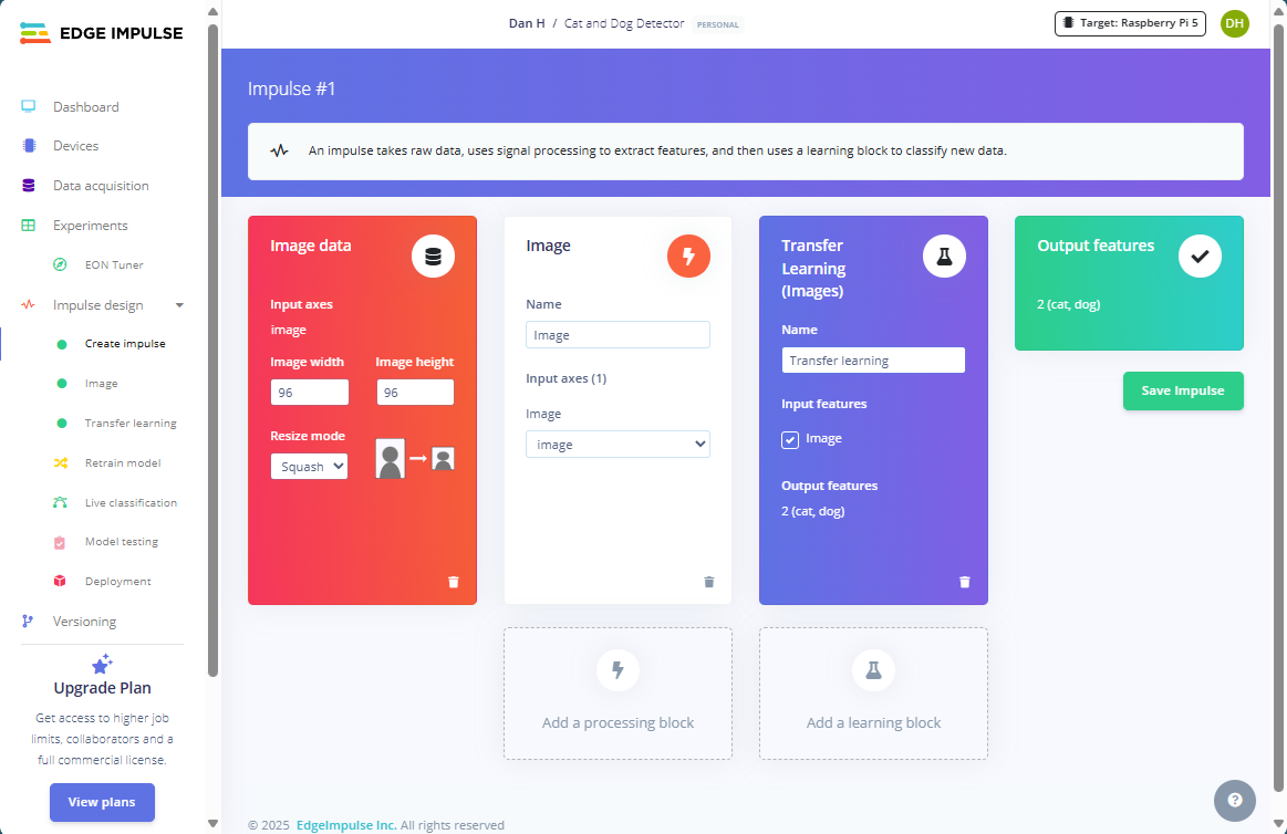
Figure 1: Create a new impulse
Don’t forget to save the impulse before proceeding. Then, click “Image” right underneath “Create Impulse” in the left toolbar to adjust the feature extraction block. Tick the “grayscale” checkbox in the “Parameters” tab. Then, navigate to the “Generate Features” tab and use the button to start feature generation. After a while, you should see a 2D-plot of the feature explorer:
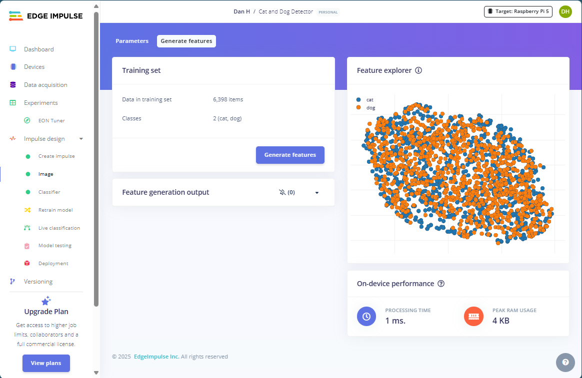
Figure 2: Extract features from the images
The image feature extractor resizes all input images, converts them to grayscale, and then turns the pixel information into a feature vector. In this instance, each image is converted to a vector of length 96x96x1 (width x height x colors). For the visualization, the features are reduced to two dimensions.
Interpreting Feature Plots
Unfortunately, the plot reveals that the two classes are not separating well. You can see that because the orange and blue dots representing samples of the two classes do not form any distinct clusters. Instead, they are just mixed. To make matters worse, neither of the classes seems to follow any observable shape or pattern in the visualization. Instead, it’s just two intermixed blobs, hinting toward a few possible problems:
- The data may not be linearly separable
In this case, we would need to increase the dimensionality or re-evaluate the labels if they overlap - Poor feature representation / Noise in the data
Here, we have to investigate the data and ensure that the samples clearly show what is relevant to the target label - Improper feature extraction / Insufficient preprocessing
The only thing we could do here is to use different approaches
However, you must remember that the 2D plot may not adequately represent the separation of the classes in higher dimensions. The two classes may still be separable in a higher dimensional space. So, while this situation is not ideal, it also doesn’t necessarily ring any alarm bells at this point, and we should still proceed with training to see how the model performs (especially since it won’t take that long).
Training the Model in Edge Impulse
After feature extraction, click the “Transfer Learning” option in the left toolbar and start the training process without changing any options. After a few minutes, you should see something like this:
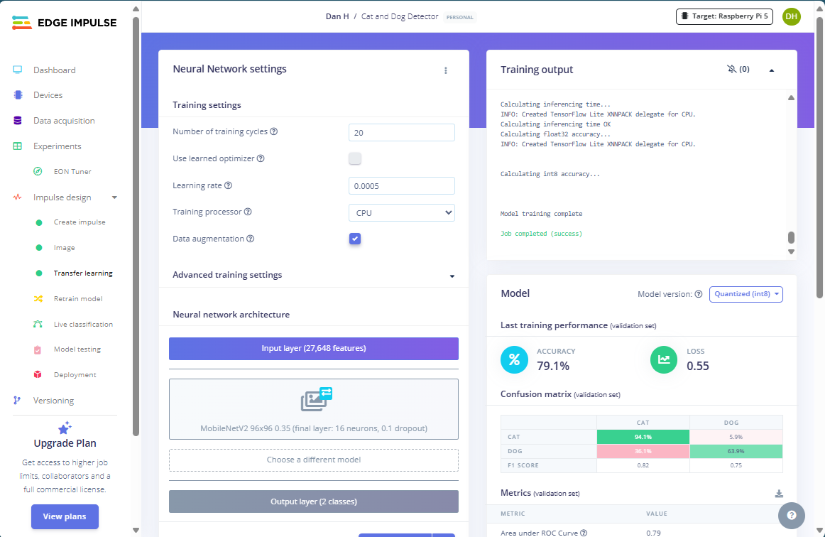
The average model accuracy is 80%, which is not horrendous but also far from what we should be able to achieve realistically (at least 95%). A closer look at the confusion matrix reveals that the model did well when predicting cat images with an accuracy of 96%. Still, in 36% of the cases where an image showed a dog, the model misclassified it as one showing a cat. To me, this indicates overfitting to the cat class either because:
- There are not enough dog samples compared to cat samples
Not the case here - Dog images do not show enough distinct features that distinguish them from cat images
Likely, we need to enhance feature representation - Dog images contain noise or mislabeled cat images
Maybe, we need to take a closer look at the data - Dogs breeds may just look much more different to one another vs. cats
Then, we should think about focusing on representative samples
Addressing Model Performance Issues
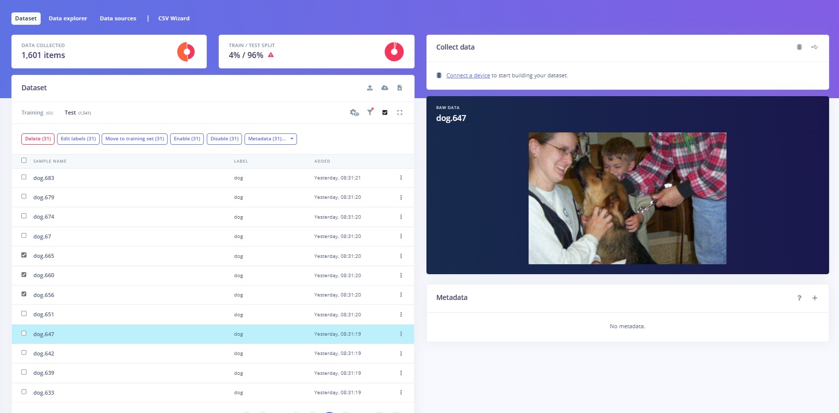
I suspect the data set we used may be too large for its own good. It may contain too many samples and reach the point where it actually dilutes the distinguishing features that differentiate cats from dogs. So, we need to concentrate the samples to ensure that the model learns what is significant when deciding whether an image shows a cat or a dog. There may also be too many small or blurry images of dogs in the set, resulting in upscaled and noisy samples compared to cleaner cat images.
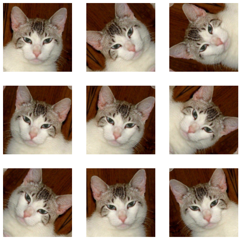
To address the problems, I’ll start by removing all but 75 training samples of each class from the data panel. I then manually perform an 80-20 split and repeat the feature extraction process. While selecting samples, I noticed that many images of dogs were taken in portrait mode (vs. landscape cat images), and they often contained other objects or people that diluted the features the model should focus on (i.e., the dog itself):
After selecting more representative samples, the model learns to cluster images based on whether they show a cat or a dog much more effectively, with an average accuracy of 90% (which is acceptable when using only 60 samples for training):
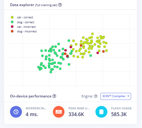
This issue highlights the importance of good data selection and preprocessing. Selecting representative samples is vital. However, you must also select a diverse set of sample images, ideally showing the subject of interest from multiple angles, lighting conditions, etc., to ensure the model does not overfit or learn some arbitrary pattern. For example, many images of dogs are taken outdoors. Cat images usually show indoor spaces. A model could learn that green grass or higher exposure equals an image that shows a dog, even though those two factors have nothing to do with dogs.
Data augmentation can help tackle overfitting in small data sets, and the feature is enabled by default when performing transfer learning. This approach slightly varies input images to generate more samples. Slight variations can include rotating the image, scaling it, zooming in or out, cropping, changing the contrast, adjusting the exposure, etc.
Postprocessing and Quantization
As a final remark, you may have noticed that the final step of model training consists of quantization. What is that? Similar to how we pre-processed images before feeding them into the model for training and classification, we can also post-process the created model to reduce its size and complexity in a process called quantization. In simple terms, quantization transforms the data format used to represent numbers within the trained model from a more precise one (e.g., float-32) to a simpler but less precise one (e.g., int-8). In doing so, the model suffers a usually negligible loss in accuracy when predicting labels on new data. However, in return, the model takes up less storage space, and inference is typically quicker, especially on more limited hardware, such as embedded microprocessors.
Classifying Unseen Images
Finally, it’s time to test the model with images it has never seen before. In practice, this data would come from sensors, such as a camera. However, we can simulate a camera by uploading a static image to edge impulse.
We can then let the model decide whether an image contains a cat or a dog. To do so, navigate to the “Model Testing” tab using the left toolbar, and then click the “Classify all” button to run inference on all test images. The model classifies each of them, and the website displays a list of all results so you can inspect which ones were misclassified by the model:
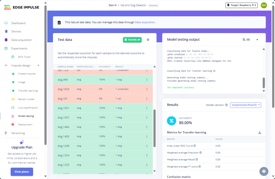
The model is about 80% accurate using the test data, which is far from perfect but acceptable given the limited data set. Out of five mistakes, only three were misclassified, and in two instances, the model could not decide whether the image shows a dog or a cat.
Table of Contents
Part 1 - AI Made Accessible: Model Training for Beginners with Edge Impulse
Part 2 - Build a Professional Machine-Learning Model in Minutes Without Programming (You are here)